RPACT Training for FGK
July 22, 2025
Welcome to the RPACT Training 2025!
This website is accessible at fgk.rpact.com
Overview
- Interim Analyse ohne Fallzahlanpassung
- Interim Analyse mit verblindeter Fallzahlanpassung
- Fallzahlanpassung basierend auf entblindeter Varianz
- Multi-arm trials
- Herleitung von Schätzern und Konfidenzintervallen
- Praktische Beispiele für:
- Cochran-Mantel-Haenszel Test: Common Odds Ratio inklusive Konfidenzintervall
- Lineares Model: LS-Means mit Konfidenzintervall und Konfidenzintervall der Differenz
Questions and Answers
Interim Analyse ohne Fallzahlanpassung
- Überprüfung der Safety (z.B. AEs), keine weiteren Anpassungen
Wird dies als Fixed Design bezeichnet? Oder ist die Bezeichnung egal?
Design mit safety monitoring
Muss etwas bei der Studienplanung berücksichtigt werden?
Organisation eines DSMBs (charter, etc.)
Interim Analyse ohne Fallzahlanpassung
- Non-binding futility, kein Test auf Efficacy:
Nennt man das bereits gruppensequentielles Design?
Ja, es ist ein gruppensequentielles Design, da eine IA geplant ist.
Dürfte so eine Studie wie ein Fixed Design geplant werden? Oder muss die IA berücksichtigt werden, bezahlt man in irgendeiner Form dafür (z.B. Power)?
Bei Planung sollte futility stop berücksichtigt werden (power!)
Wenn der p-Wert für die Futility Entscheidung verwendet wird (also z.B. Stop für Futility für p > 0.9), muss bei der finalen Analyse dafür adjustiert werden?
Nein bei non-binding futility, man kann bei binding futility.
Interim Analyse ohne Fallzahlanpassung
- Non-binding futility, Test auf Efficacy:
Alpha-spending: theoretisch darf man den Zeitpunkt und die Anzahl an Zwischenauswertungen anpassen. Wird es von Behörden akzeptiert, Anzahl und Zeitpunkt der Zwischenauswertung nicht im Protokoll zu präspezifizieren?
Bei Verwendung des alpha spending Ansatzes sollte Zeitpunkt spezifiziert werden, information bei IA ist flexibel. Zeitpunkt darf nicht (datanabhängig) angepasst werden, wenn alpha spending verwendet wird.
Welchen Mehrwert hat es einen Test auf Efficacy einzubauen, wenn die Chance für einen Abbruch bei der IA minimal ist (z.B. mit O‘Brien Fleming Design)? Gibt es einen sinnvollen Anwendungsfall bzw. welche Daseinsberechtigung hat ein O‘Brien Fleming Design?
O’Brien Fleming design ist sehr etablierte Methode, die von Behörden akzeptiert wird. Für minimale Abruchchance mit minimalen Kosten verbaut man sich nichts!
Interim Analyse mit verblindeter Fallzahlanpassung
- Kein Test auf Futility/Efficacy:
„Bezahlt“ man für so eine Analyse? Man kann gepoolt auswerten und hat kein alpha Adjustment.
Type I error rate inflation muss diskutiert werden
Nachteile:
- Fallzahlneuberechnung kann irreführend sein
- Bräuchte es ein IDMC?
- Gibt es weitere Nachteile?
Wann irreführend? IDMC ist nicht notwendig, da keine Entscheidung getroffen wird
Müsste ein Check auf Futility (non-binding) in irgendeiner Form bei der Auswertung berücksichtigt werden?
Verblindete Fallzahlanpassung und futility check schließen sich aus
Fallzahlanpassung basierend auf entblindeter Varianz
- Kein Test auf Efficacy, ggf. auch Check auf Futility:
Dürfen bei einigermaßen großer Fallzahl die Daten gepoolt und ohne alpha Adjustment ausgewertet werden? Gibt es eine Daumenregel?
Definitiv nein, ich weiß ja nicht, wie die große Fallzahl entstanden ist!
- Test auf Efficacy, ggf. auch Check auf Futility:
Dürfen die Daten gepoolt ausgewertet werden?
Promizing zone approach: wenn bedingte power > 50% kann Fallzahl erhöht und gepoolt ausgewertet werden
Ist ein alpha Adjustment für den Efficacy Test ausreichend oder ist eine weitere Adjustierung aufgrund der Fallzahlanpassung notwendig?
Weitere Anpassung i.A. nötig
Multi-arm trials
- 3-armige Studie mit zwei Dosisgruppen; es wird nur die bessere Verumgruppe nach der IA weitergeführt:
Muss die finale Auswertung mit der inversen Normalmethode erfolgen?
Nicht muss, aber gute Anwendung. Bei festen Selektionsregeln gibt es andere Verfahren, die aber m.E. wenig Vorteile bringen
Ohne Test auf Efficacy bei der IA: ist eine alpha Adjustierung für die IA notwendig?
Bitte diese Frage näher spezifizieren
Allgemeines
Wie wirkt es sich aus, wenn wir kein superiority sondern ein non-inferiority trial haben?
Bitte auch diese Frage näher spezifizieren
Herleitung von Schätzern und Konfidenzintervallen
- Allgemeine Einführung welche Punkt-Schätzer es gibt und was man berücksichtigen muss
- Wie werden Konfidenzintervalle für die Punktschätzer hergeleitet?
- Praktische Beispiele für:
- Cochran-Mantel-Haenszel Test: Common Odds Ratio inklusive Konfidenzintervall
- Lineares Model: LS-Means mit Konfidenzintervall und Konfidenzintervall der Differenz
Vorschläge für Erweiterungen in rpact
- Cochran-Mantel-Haenszel Test (Auswertung und Fallzahlanpassung mit Common Odds Ratio)
- Wilcoxon Rangsummentest (Auswertung und Fallzahlanpassung)
Estimation and p-Values in Group Sequential Designs
- p-values:
- stagewise \(p\)-values
- Cumulative \(p\)-values
- Final analysis adjusted (“exact”) \(p\)-values
- Repeated \(p\,\)-values
- Estimation:
- Unadjusted CIs
- Final analysis adjusted (“exact”) CIs based on stagewise ordering
- Repeated Confidence Intervals (RCIs)
- Point estimates
Exact p-values: Ordering of sample space
In a fixed-sample design, a \(p\)-value is defined as
\[p = P_{H_0}(Z \geq z)\;.\]
In a group sequential design, define overall \(p\)-value at the end of the trial through
\[p_\text{final} = P_{H_0}\big((Z^*_{\cal K}, {\cal K}) \succeq (z^*_k,k)\big)\;.\]
Needs ordering of the sample space
Focus on methods based on stagewise ordering of group-sequential sample space:
- Good theoretical properties
- Available in software (rpact, EaSt, etc.)
Example four-stage design, two-sided test
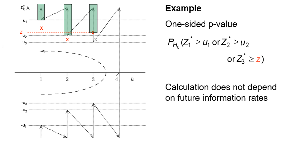
This \(p\)-value can only be calculated once, at the end of the trial
Overall repeated p-values
- The overall repeated \(p\,\)-value is the smallest significance level for which \(H_0\) can be rejected at stage \(k\) with the given data.
- Repeated \(p\,\)-values can be calculated at any stage of the trial.
- Repeated \(p\,\)-values exactly correspond to the test decision.
- Under \(H_0\), distribution of repeated \(p\,\)-value stochastically larger than uniform.
- Repeated \(p\,\)-values are conservative.
Confidence intervals and estimates
Confidence intervals:
- Repeated confidence intervals: sequence of intervals \(I_k\) for which
\[ P_\delta(\delta \in I_k \text{ for all } k = 1,\ldots,K) \geq 1 - \alpha \]
- Final analysis adjusted confidence interval, calculated by:
\[ P_{\delta^L}\big((Z^*_{\cal K}, {\cal K}) \succeq (z^*_k,k)\big) = \alpha/2 \text{ and } P_{\delta^U}\big((Z^*_{\cal K}, {\cal K}) \preceq (z^*_k,k)\big) = \alpha/2 \]
Point estimates:
Median unbiased estimator: Upper limit of a one-sided 50% confidence interval of the form \((-\infty; \delta_{0.5}]\).
Mid-point of RCI
Group Sequential and Adaptive Analysis with rpact
Analysing a Trial with Interim Stages Using rpact
- Group sequential test
- Inverse normal combination test
- Fisher’s combination test
- Repeated confidence intervals, p-Values
- Final analysis adjusted confidence intervals, p-Values
- Conditional Rejection Probability (Müller & Schäfer)
- Conditional power assessment
- All this for continuous, binary, and survival endpoint
Group Sequential and Adaptive Analysis
design The trial design.
dataInput The summary data used for calculating the test results. This is either an element of DataSetMeans, of DataSetRates, or of DataSetSurvival.
Given a design and a dataset, at given stage the function calculates the test results (effect sizes, stage-wise test statistics and p-values, overall p-values and test statistics, conditional rejection probability (CRP), conditional power, Repeated Confidence Intervals (RCIs), repeated overall p-values, and final stage p-values, median unbiased effect estimates, and confidence intervals.)
The conditional power is calculated only if (at least) the sample size for the subsequent stage(s) is specified. Median unbiased effect estimates and confidence intervals are calculated only if a group sequential or an inverse normal design was chosen. A final stage \(p\)-value for Fisher’s combination test is calculated only if a two-stage design was chosen.
Group Sequential and Adaptive Analysis
dataInput
An element of
DataSetMeansfor one sample is created bygetDataset(means =, stDevs =, sampleSizes =)where
means, stDevs, sampleSizesare vectors with stagewise means, standard deviations, and sample sizes of length given by the number of available stages.
An element of
DataSetMeansfor two samples is created bygetDataset(means1 =, means2 =, stDevs1 =, stDevs2 =, sampleSizes1 =, sampleSizes2 =)where
means1, means2, stDevs1, stDevs2, sampleSizes1, sampleSizes2are vectors with stagewise means, standard deviations, and sample sizes for the two treatment groups of length given by the number of available stages.
Use of cumMeans, cumulativeMeans, overallMeans, cumStDevs, cumulativeStDevs, overallStDevs, n, cumN, etc., is also possible
Group Sequential and Adaptive Analysis
dataInput
An element of
DataSetMeansfor G + 1 samples is created bygetDataset(means1 =,..., means[G+1] =, stDevs1 =, ...,stDevs[G+1] =, sampleSizes1 =, ..., sampleSizes[G+1] =),where
means1, ..., means[G+1], stDevs1, ..., stDevs[G+1], sampleSizes1, ..., sampleSizes[G+1]are vectors with stagewise means, standard deviations, and sample sizes for G+1 treatment groups of length given by the number of available stages.Last treatment arm G + 1 always refers to the control group that cannot be deselected.
Only for the first stage all treatment arms needs to be specified, so treatment arm selection with an arbitrary number of treatment arms for subsequent stage can be considered.
Analogue definition of
DataSetRatesandDataSetSurvival.
Example
Define the design:
Data summary for binary data:
Analysis results
getAnalysisResults(
  design = designIN,
  dataInput = dataExample,
  directionUpper = FALSE
) |> summary()
Analysis results for a binary endpoint
Sequential analysis with 4 looks (inverse normal combination test design), one-sided overall significance level 2.5%. The results were calculated using a two-sample test for rates, normal approximation test. H0: pi(1) - pi(2) = 0 against H1: pi(1) - pi(2) < 0.
| Stage | 1 | 2 | 3 | 4 |
|---|---|---|---|---|
| Fixed weight | 0.5 | 0.5 | 0.5 | 0.5 |
| Cumulative alpha spent | 0.0070 | 0.0138 | 0.0198 | 0.0250 |
| Stage levels (one-sided) | 0.0070 | 0.0088 | 0.0100 | 0.0110 |
| Efficacy boundary (z-value scale) | 2.456 | 2.372 | 2.325 | 2.291 |
| Cumulative effect size | -0.352 | -0.361 | -0.389 | |
| Cumulative treatment rate | 0.375 | 0.389 | 0.444 | |
| Cumulative control rate | 0.727 | 0.750 | 0.833 | |
| Stage-wise test statistic | -1.536 | -1.799 | -2.567 | |
| Stage-wise p-value | 0.0623 | 0.0360 | 0.0051 | |
| Inverse normal combination | 1.536 | 2.358 | 3.407 | |
| Test action | continue | continue | reject and stop | |
| Conditional rejection probability | 0.0777 | 0.3093 | 0.9062 | |
| 95% repeated confidence interval | [-0.739; 0.197] | [-0.646; 0.002] | [-0.618; -0.140] | |
| Repeated p-value | 0.1561 | 0.0259 | 0.0009 | |
| Final p-value | 0.0139 | |||
| Final confidence interval | [-0.598; -0.039] | |||
| Median unbiased estimate | -0.333 |
Check repeated p-value
getAnalysisResults(
  design = getDesignInverseNormal(
      kMax = 4,
      alpha = 0.02595,
      typeOfDesign = "WT",
      deltaWT = 0.45
    ),
  dataInput = dataExample,
  directionUpper = FALSE
) |> summary()
Analysis results for a binary endpoint
Sequential analysis with 4 looks (inverse normal combination test design), one-sided overall significance level 2.6%. The results were calculated using a two-sample test for rates, normal approximation test. H0: pi(1) - pi(2) = 0 against H1: pi(1) - pi(2) < 0.
| Stage | 1 | 2 | 3 | 4 |
|---|---|---|---|---|
| Fixed weight | 0.5 | 0.5 | 0.5 | 0.5 |
| Cumulative alpha spent | 0.0073 | 0.0144 | 0.0206 | 0.0260 |
| Stage levels (one-sided) | 0.0073 | 0.0092 | 0.0104 | 0.0114 |
| Efficacy boundary (z-value scale) | 2.440 | 2.357 | 2.310 | 2.277 |
| Cumulative effect size | -0.352 | -0.361 | -0.389 | |
| Cumulative treatment rate | 0.375 | 0.389 | 0.444 | |
| Cumulative control rate | 0.727 | 0.750 | 0.833 | |
| Stage-wise test statistic | -1.536 | -1.799 | -2.567 | |
| Stage-wise p-value | 0.0623 | 0.0360 | 0.0051 | |
| Inverse normal combination | 1.536 | 2.358 | 3.407 | |
| Test action | continue | reject and stop | reject and stop | |
| Conditional rejection probability | 0.0806 | 0.3181 | 0.9110 | |
| 94.81% repeated confidence interval | [-0.737; 0.194] | [-0.644; 0.000] | [-0.617; -0.142] | |
| Repeated p-value | 0.1561 | 0.0259 | 0.0009 | |
| Final p-value | 0.0144 | |||
| Final confidence interval | [-0.656; -0.041] | |||
| Median unbiased estimate | -0.354 |
Check RCI
getAnalysisResults(
  design = designIN,
  dataInput = dataExample,
  thetaH0 = 0.0025,  #  output is rounded!
  directionUpper = FALSE
) |> summary()
Analysis results for a binary endpoint
Sequential analysis with 4 looks (inverse normal combination test design), one-sided overall significance level 2.5%. The results were calculated using a two-sample test for rates, normal approximation test. H0: pi(1) - pi(2) = 0.0025 against H1: pi(1) - pi(2) < 0.0025.
| Stage | 1 | 2 | 3 | 4 |
|---|---|---|---|---|
| Fixed weight | 0.5 | 0.5 | 0.5 | 0.5 |
| Cumulative alpha spent | 0.0070 | 0.0138 | 0.0198 | 0.0250 |
| Stage levels (one-sided) | 0.0070 | 0.0088 | 0.0100 | 0.0110 |
| Efficacy boundary (z-value scale) | 2.456 | 2.372 | 2.325 | 2.291 |
| Cumulative effect size | -0.352 | -0.361 | -0.389 | |
| Cumulative treatment rate | 0.375 | 0.389 | 0.444 | |
| Cumulative control rate | 0.727 | 0.750 | 0.833 | |
| Stage-wise test statistic | -1.547 | -1.811 | -2.577 | |
| Stage-wise p-value | 0.0610 | 0.0351 | 0.0050 | |
| Inverse normal combination | 1.547 | 2.374 | 3.427 | |
| Test action | continue | reject and stop | reject and stop | |
| Conditional rejection probability | 0.0790 | 0.3170 | 0.9118 | |
| 95% repeated confidence interval | [-0.739; 0.197] | [-0.646; 0.002] | [-0.618; -0.140] | |
| Repeated p-value | 0.1534 | 0.0249 | 0.0008 | |
| Final p-value | 0.0138 | |||
| Final confidence interval | [-0.658; -0.039] | |||
| Median unbiased estimate | -0.354 |
Comparison of point estimates
Testing means
Testing means
Analysis results for a continuous endpoint
Sequential analysis with 4 looks (inverse normal combination test design), one-sided overall significance level 2.5%. The results were calculated using a one-sample t-test. H0: mu = 0 against H1: mu > 0.
| Stage | 1 | 2 | 3 | 4 |
|---|---|---|---|---|
| Fixed weight | 0.5 | 0.5 | 0.5 | 0.5 |
| Cumulative alpha spent | 0.0070 | 0.0138 | 0.0198 | 0.0250 |
| Stage levels (one-sided) | 0.0070 | 0.0088 | 0.0100 | 0.0110 |
| Efficacy boundary (z-value scale) | 2.456 | 2.372 | 2.325 | 2.291 |
| Cumulative effect size | 0.330 | 0.383 | 0.379 | |
| Cumulative standard deviation | 0.970 | 0.941 | 0.918 | |
| Stage-wise test statistic | 1.800 | 2.856 | 2.264 | |
| Stage-wise p-value | 0.0415 | 0.0034 | 0.0157 | |
| Inverse normal combination | 1.733 | 3.138 | 3.804 | |
| Test action | continue | reject and stop | reject and stop | |
| Conditional rejection probability | 0.1040 | 0.7069 | 0.9776 | |
| 95% repeated confidence interval | [-0.151; 0.811] | [0.097; 0.662] | [0.152; 0.601] | |
| Repeated p-value | 0.1120 | 0.0028 | 0.0002 | |
| Final p-value | 0.0075 | |||
| Final confidence interval | [0.077; 0.577] | |||
| Median unbiased estimate | 0.342 |
[1] 0.3300000 0.3829412 0.3790722 NA[1] NA 0.3422945 NA NA[1] 0.3300000 0.3799040 0.3766444 NACovariate Adjusted Analysis
Introduction
Compute adjusted means and estimated standard deviations for continuous outcomes in a two-armed trial with covariates.
Perform group sequential test with adjusted p-values from ANCOVA.
Use the function
getDataset()as an utility function to process adjusted means and estimated standard deviations from raw data.This is done through the extraction of
lmcoefficients from the specified ANCOVA.
Analysis of raw data – Data import from csv file
Artificial dataset that was randomly generated with simulated normal data.
The dataset has six variables:
- Subject id
- Stage number
- Group name
- An example
outcomein that we are interested in - The first covariate
gender - The second covariate
covariate
subject stage group outcome gender covariate
1 1101 1 Treatment group 60.915332 m 41.74395
2 1102 1 Treatment group 57.651981 f 43.94315
3 1103 1 Treatment group 118.367548 f 38.82385
4 1104 1 Treatment group 118.251238 m 36.79198
5 1105 1 Treatment group 174.353213 f 42.92030
6 1106 1 Treatment group 113.806819 f 36.30031
7 1107 1 Treatment group 48.692310 m 38.79058
8 1108 1 Treatment group 120.793274 f 41.98949
9 1109 1 Treatment group 102.074481 m 43.56432
10 1110 1 Treatment group 66.653356 m 41.28624
11 1111 1 Treatment group 192.789917 m 33.28636
12 1112 1 Treatment group 96.103188 f 46.12874
13 1113 1 Treatment group 175.411482 m 45.50095
14 1114 1 Treatment group 179.898767 m 33.24516
15 1115 1 Treatment group 64.836731 f 41.73938
16 1116 1 Treatment group 138.559278 m 45.31195
17 1117 1 Treatment group 29.529644 m 35.75133
18 1118 1 Treatment group 122.545254 f 42.96523
19 1119 1 Treatment group 128.296674 f 44.73482
20 1120 1 Treatment group 110.110602 f 44.49367
21 1121 1 Treatment group 45.991520 f 33.88518
22 1122 1 Treatment group 87.296190 m 36.73631
23 1123 1 Treatment group 92.254379 f 38.08448
24 1124 1 Treatment group 96.479000 f 41.33588
25 1125 1 Treatment group 97.732579 m 44.31532
26 1126 1 Treatment group 63.020381 m 38.82376
27 1127 1 Treatment group 236.277237 f 41.20683
28 1128 1 Treatment group NA m 42.33282
29 1129 1 Treatment group 45.273090 m 43.90040
30 1130 1 Treatment group 56.091711 m 39.27349
31 1131 1 Treatment group 134.051026 f 39.04124
32 1132 1 Treatment group 97.138590 f 44.51122
33 1133 1 Treatment group 106.926291 m 34.70051
34 1134 1 Treatment group 68.084850 m 38.63797
35 1135 1 Treatment group 135.710674 m 35.48387
36 1136 1 Treatment group 172.006534 m 43.41109
37 1137 1 Treatment group 79.420273 f 52.92393
38 1138 1 Treatment group 88.884478 m 39.24610
39 1139 1 Treatment group 72.875501 m 43.17024
40 1140 1 Treatment group 62.499853 m 35.90245
41 1141 1 Treatment group 112.013073 m 35.75578
42 1142 1 Treatment group 108.973606 f 37.57677
43 1143 1 Treatment group NA f 38.43325
44 1144 1 Treatment group 108.609868 m 44.35666
45 1145 1 Treatment group 196.333999 f 42.28084
46 1146 1 Treatment group 95.173415 f 39.94827
47 1147 1 Treatment group 31.068515 m 40.39852
48 1148 1 Treatment group NA f 37.29137
49 1149 1 Treatment group 84.588106 f 42.04340
50 1150 1 Treatment group 128.541775 m 44.99807
51 1151 1 Treatment group 118.149249 m 40.69396
52 1152 1 Treatment group 108.698464 m 45.93401
53 1153 1 Treatment group 66.551613 m 39.51589
54 1154 1 Treatment group 66.795196 m 37.24943
55 1155 1 Treatment group 148.194515 f 41.63981
56 1156 1 Treatment group 97.581556 m 43.30963
57 1157 1 Treatment group 87.086105 f 44.24383
58 1158 1 Treatment group 75.265103 m 48.30317
59 1159 1 Treatment group 115.077812 f 44.97853
60 1160 1 Treatment group 215.990333 m 37.98066
61 1161 1 Treatment group 83.430914 f 37.53304
62 1162 1 Treatment group 133.453484 f 33.68154
63 1163 1 Treatment group 139.787199 f 41.92989
64 1164 1 Treatment group 189.090864 m 47.64797
65 1165 1 Treatment group 96.461852 f 34.88215
66 1166 1 Treatment group 149.629258 m 34.87189
67 1167 1 Treatment group 87.983660 m 37.79579
68 1168 1 Treatment group 125.487429 f 39.74570
69 1169 1 Treatment group 49.868054 f 40.15935
70 1170 1 Treatment group 111.678537 m 41.74537
71 1171 1 Treatment group 155.733073 m 37.03043
72 1172 1 Treatment group 89.898656 f 38.49887
73 1173 1 Treatment group 133.281809 m 38.02761
74 1174 1 Treatment group 180.787879 f 37.27137
75 1175 1 Treatment group 181.326264 f 42.22095
76 1176 1 Treatment group 46.644730 f 34.46649
77 1177 1 Treatment group 182.160889 m 44.23738
78 1178 1 Treatment group 235.734964 f 44.07047
79 1179 1 Treatment group 123.596910 f 39.80186
80 1180 1 Treatment group 100.572744 f 31.83763
81 1181 1 Treatment group 79.068517 m 39.61799
82 1182 1 Treatment group 119.959232 m 39.33848
83 1183 1 Treatment group 79.618169 m 42.26236
84 1184 1 Treatment group 101.267554 f 38.10153
85 1185 1 Treatment group 85.285744 m 43.76071
86 1186 1 Treatment group 125.969216 m 37.75873
87 1187 1 Treatment group 104.409242 m 46.81732
88 1201 1 Control group 118.111978 f 46.37750
89 1202 1 Control group 112.803047 f 50.56341
90 1203 1 Control group 106.279228 m 46.16517
91 1204 1 Control group 26.137107 m 55.66513
92 1205 1 Control group 121.703709 m 46.10107
93 1206 1 Control group 28.179089 f 47.32115
94 1207 1 Control group 166.258299 m 50.56693
95 1208 1 Control group 93.908330 m 48.99593
96 1209 1 Control group 117.873985 f 44.74084
97 1210 1 Control group 77.797407 m 51.11756
98 1211 1 Control group 97.793048 f 45.79823
99 1212 1 Control group 34.490830 f 47.80869
100 1213 1 Control group 108.603770 m 55.23996
101 1214 1 Control group 80.016652 f 54.73093
102 1215 1 Control group 180.938509 m 49.60275
103 1216 1 Control group 119.506045 f 48.43063
104 1217 1 Control group 130.953498 m 45.92114
105 1218 1 Control group -51.531817 f 49.71211
106 1219 1 Control group 140.740705 f 46.09804
107 1220 1 Control group 83.788848 f 57.85032
108 1221 1 Control group 73.960984 m 51.60963
109 1222 1 Control group 41.871488 m 44.46589
110 1223 1 Control group 87.101741 m 48.91804
111 1224 1 Control group 21.869485 m 54.32146
112 1225 1 Control group 130.166118 f 45.12141
113 1226 1 Control group 123.082088 m 50.82517
114 1227 1 Control group 142.370876 f 46.80575
115 1228 1 Control group 65.328749 f 56.64114
116 1229 1 Control group 118.455944 f 48.18142
117 1230 1 Control group 141.864325 m 48.35794
118 1231 1 Control group 74.501536 f 54.57813
119 1232 1 Control group 41.971384 m 44.73958
120 1233 1 Control group 114.503414 f 46.72186
121 1234 1 Control group 166.778918 f 53.91904
122 1235 1 Control group 107.779407 m 48.52357
123 1236 1 Control group 141.209154 f 53.76970
124 1237 1 Control group 85.258166 m 49.97739
125 1238 1 Control group 123.324872 f 58.23043
126 1239 1 Control group 106.191564 m 48.04120
127 1240 1 Control group 136.704361 f 49.95438
128 1241 1 Control group 168.320594 f 49.83972
129 1242 1 Control group 191.833899 f 44.82796
130 1243 1 Control group 41.993953 f 47.82318
131 1244 1 Control group 122.223310 m 51.26559
132 1245 1 Control group 107.417838 f 41.08096
133 1246 1 Control group 66.660155 f 44.16594
134 1247 1 Control group 118.630493 f 49.50234
135 1248 1 Control group 103.357250 m 50.14601
136 1249 1 Control group 68.091491 m 47.21945
137 1250 1 Control group 197.232504 m 52.14219
138 1251 1 Control group 55.352899 f 52.05785
139 1252 1 Control group 95.254020 f 55.60368
140 1253 1 Control group 84.331326 f 45.64885
141 1254 1 Control group 55.833782 m 49.94821
142 1255 1 Control group -25.137811 m 54.53565
143 1256 1 Control group 58.127828 f 59.07245
144 1257 1 Control group 62.478912 m 56.62178
145 1258 1 Control group 106.973422 f 44.66975
146 1259 1 Control group 110.471942 f 56.09414
147 1260 1 Control group 113.071582 m 54.36411
148 1261 1 Control group 64.365801 m 44.54071
149 1262 1 Control group 88.582148 m 51.48605
150 1263 1 Control group 108.000380 f 48.18828
151 1264 1 Control group 107.973560 f 49.99834
152 1265 1 Control group 19.778149 f 50.24998
153 1266 1 Control group 181.203995 f 50.44074
154 1267 1 Control group 144.530158 f 48.07444
155 1268 1 Control group 138.653984 f 45.89275
156 1269 1 Control group -13.645824 f 46.27012
157 1270 1 Control group 70.376653 f 54.58227
158 1271 1 Control group 79.519125 f 49.23130
159 1272 1 Control group 23.968025 f 50.48166
160 1273 1 Control group 146.145097 f 47.41035
161 1274 1 Control group 75.505468 m 54.12894
162 1275 1 Control group 64.769655 m 51.41633
163 1276 1 Control group 44.061803 m 50.83071
164 1277 1 Control group 62.239958 m 56.12589
165 1278 1 Control group 96.003713 m 51.44122
166 1279 1 Control group 158.426362 m 43.78677
167 1280 1 Control group 28.771248 m 50.45153
168 1281 1 Control group 75.185158 f 51.54136
169 1282 1 Control group -27.140455 m 51.43388
170 1283 1 Control group 74.475666 m 50.67419
171 1284 1 Control group 103.817718 m 45.48959
172 1285 1 Control group 61.775227 m 56.85924
173 1286 1 Control group 114.031613 m 44.89346
174 1287 1 Control group 42.393840 m 52.27747
175 2101 2 Treatment group 148.131778 m 33.76559
176 2102 2 Treatment group 96.019897 f 40.68627
177 2103 2 Treatment group NA f 43.29108
178 2104 2 Treatment group NA m 39.47415
179 2105 2 Treatment group 124.068427 f 41.29759
180 2106 2 Treatment group 226.969836 m 41.12901
181 2107 2 Treatment group 123.405054 m 43.50771
182 2108 2 Treatment group NA m 37.00055
183 2109 2 Treatment group 101.649519 m 41.92557
184 2110 2 Treatment group 152.672985 m 36.02520
185 2111 2 Treatment group 129.906677 m 46.45029
186 2112 2 Treatment group 101.838703 m 35.06772
187 2113 2 Treatment group 69.199847 f 36.18072
188 2114 2 Treatment group 185.983430 m 38.82010
189 2115 2 Treatment group 54.855420 m 41.00171
190 2116 2 Treatment group 195.816339 f 44.44986
191 2117 2 Treatment group 148.873317 m 43.99352
192 2118 2 Treatment group 73.546096 f 38.59094
193 2119 2 Treatment group 131.324795 m 41.23274
194 2120 2 Treatment group 70.147824 m 41.09979
195 2121 2 Treatment group 165.142632 m 38.58412
196 2122 2 Treatment group 63.119932 m 43.86155
197 2123 2 Treatment group 113.534704 m 40.48399
198 2124 2 Treatment group 56.760798 m 41.35577
199 2125 2 Treatment group 113.147409 m 43.40006
200 2126 2 Treatment group 161.692264 f 41.28116
201 2127 2 Treatment group NA m 38.61404
202 2128 2 Treatment group 144.895706 m 40.52785
203 2129 2 Treatment group 120.076608 m 40.93657
204 2130 2 Treatment group 167.198650 m 37.69830
205 2131 2 Treatment group 92.370218 f 42.38907
206 2132 2 Treatment group 174.970652 f 42.71503
207 2133 2 Treatment group 43.700108 f 36.92546
208 2134 2 Treatment group 86.721918 f 38.58603
209 2135 2 Treatment group 173.329034 m 36.65433
210 2136 2 Treatment group 68.955282 m 46.10965
211 2137 2 Treatment group -13.494525 m 44.82764
212 2138 2 Treatment group -12.219344 m 45.74248
213 2139 2 Treatment group 93.200749 f 33.26283
214 2140 2 Treatment group 127.781442 f 41.19897
215 2141 2 Treatment group 99.416015 m 39.88825
216 2142 2 Treatment group 83.291346 f 40.62557
217 2143 2 Treatment group 104.417974 f 35.15310
218 2144 2 Treatment group 53.158243 m 43.69736
219 2145 2 Treatment group 131.279052 m 37.56266
220 2146 2 Treatment group 146.385221 f 46.89227
221 2147 2 Treatment group 87.871764 m 41.71479
222 2148 2 Treatment group 92.074664 f 36.69945
223 2149 2 Treatment group 145.358484 f 37.25947
224 2150 2 Treatment group 127.476922 f 42.75383
225 2151 2 Treatment group 87.122459 f 36.80236
226 2152 2 Treatment group 99.468734 m 40.72832
227 2153 2 Treatment group 116.205793 m 45.07193
228 2154 2 Treatment group 118.363383 m 36.11800
229 2155 2 Treatment group 195.779889 m 46.85061
230 2156 2 Treatment group 84.809065 f 34.89991
231 2157 2 Treatment group 122.554800 m 37.26509
232 2158 2 Treatment group 40.524856 f 40.69914
233 2159 2 Treatment group 75.646884 m 37.54613
234 2160 2 Treatment group 129.848641 m 41.91331
235 2161 2 Treatment group 159.660881 f 42.99501
236 2162 2 Treatment group 85.972244 f 36.97553
237 2163 2 Treatment group 54.394505 f 40.09344
238 2164 2 Treatment group 152.676684 f 41.60451
239 2165 2 Treatment group 149.225960 f 48.85437
240 2166 2 Treatment group 169.240155 f 37.02340
241 2167 2 Treatment group 155.218245 m 39.26598
242 2168 2 Treatment group NA f 31.72879
243 2169 2 Treatment group 102.263295 m 45.52036
244 2170 2 Treatment group 223.272314 m 36.12225
245 2171 2 Treatment group 161.310825 f 37.35040
246 2172 2 Treatment group 66.869670 f 41.80688
247 2173 2 Treatment group 188.059613 f 40.23286
248 2174 2 Treatment group 121.116022 m 39.61774
249 2175 2 Treatment group 64.347836 f 36.83015
250 2176 2 Treatment group 114.101965 f 31.02810
251 2177 2 Treatment group NA m 38.26138
252 2178 2 Treatment group 67.757731 m 42.71542
253 2179 2 Treatment group 131.464220 f 36.02921
254 2180 2 Treatment group 53.728041 m 42.26535
255 2181 2 Treatment group 207.710614 f 37.34099
256 2182 2 Treatment group 98.115872 f 41.14550
257 2183 2 Treatment group 146.508829 m 40.63603
258 2184 2 Treatment group NA f 37.68016
259 2185 2 Treatment group NA f 46.09672
260 2186 2 Treatment group 33.627667 m 34.10929
261 2187 2 Treatment group 88.514103 m 36.74357
262 2201 2 Control group 85.564947 f 48.77833
263 2202 2 Control group 88.082937 f 54.62074
264 2203 2 Control group 101.821924 m 47.39312
265 2204 2 Control group 69.498987 f 52.80377
266 2205 2 Control group 76.389332 f 58.28917
267 2206 2 Control group 197.718320 f 42.83755
268 2207 2 Control group 80.491819 f 52.43532
269 2208 2 Control group 88.790640 m 52.52622
270 2209 2 Control group 27.785576 f 56.67482
271 2210 2 Control group 110.395608 f 43.89054
272 2211 2 Control group 189.602362 f 55.32527
273 2212 2 Control group 116.706192 f 55.56885
274 2213 2 Control group 53.403402 m 47.87397
275 2214 2 Control group 92.197839 m 44.35599
276 2215 2 Control group 226.719523 m 48.81198
277 2216 2 Control group 84.333440 f 52.99306
278 2217 2 Control group 115.058642 m 54.70769
279 2218 2 Control group NA m 46.39091
280 2219 2 Control group 147.045933 f 44.11154
281 2220 2 Control group 145.633095 m 47.38888
282 2221 2 Control group 109.577890 m 52.24456
283 2222 2 Control group 78.273341 m 51.52679
284 2223 2 Control group 134.503543 f 54.62293
285 2224 2 Control group 94.809806 f 47.20078
286 2225 2 Control group 135.254918 f 50.73824
287 2226 2 Control group 148.096839 f 45.33651
288 2227 2 Control group 145.754822 m 52.73534
289 2228 2 Control group 98.575321 f 49.67044
290 2229 2 Control group 84.415325 f 57.12815
291 2230 2 Control group 102.888916 m 57.98899
292 2231 2 Control group 140.332164 f 55.65008
293 2232 2 Control group 8.320178 m 47.40147
294 2233 2 Control group 125.140663 f 53.81962
295 2234 2 Control group 54.703761 m 51.37802
296 2235 2 Control group 46.116927 f 51.06964
297 2236 2 Control group 92.555462 f 51.79276
298 2237 2 Control group 14.522516 m 48.26737
299 2238 2 Control group 100.949270 m 49.60221
300 2239 2 Control group 79.767910 m 49.06210
301 2240 2 Control group 90.308179 m 51.51113
302 2241 2 Control group 122.417868 f 49.19103
303 2242 2 Control group 125.701298 f 43.04404
304 2243 2 Control group 80.288039 m 48.82796
305 2244 2 Control group NA m 49.91225
306 2245 2 Control group 72.630434 f 48.91357
307 2246 2 Control group 115.662673 f 46.31431
308 2247 2 Control group 109.296894 f 54.15588
309 2248 2 Control group 165.928627 m 49.03998
310 2249 2 Control group 170.922467 f 52.29195
311 2250 2 Control group 58.384495 f 51.25386
312 2251 2 Control group 73.276353 f 45.32873
313 2252 2 Control group 140.114730 m 47.54660
314 2253 2 Control group 99.767996 f 55.15153
315 2254 2 Control group 83.453778 m 47.17067
316 2255 2 Control group 55.070047 f 48.32911
317 2256 2 Control group 137.944829 f 46.83519
318 2257 2 Control group 148.862366 f 45.56954
319 2258 2 Control group 192.977651 f 46.47892
320 2259 2 Control group NA f 47.55053
321 2260 2 Control group 126.582645 f 45.94865
322 2261 2 Control group 49.077900 m 54.33169
323 2262 2 Control group 133.681737 f 54.85075
324 2263 2 Control group NA m 49.64795
325 2264 2 Control group 142.001442 f 53.00226
326 2265 2 Control group 56.745110 f 57.85307
327 2266 2 Control group 96.816275 m 47.72682
328 2267 2 Control group 61.024866 f 53.09593
329 2268 2 Control group 150.454543 m 48.96315
330 2269 2 Control group NA m 47.66897
331 2270 2 Control group 26.374563 m 47.95530
332 2271 2 Control group 125.200981 f 45.77897
333 2272 2 Control group 48.343088 f 49.53677
334 2273 2 Control group 109.939541 m 50.17042
335 2274 2 Control group 121.184452 m 43.51048
336 2275 2 Control group 70.503523 f 43.82258
337 2276 2 Control group 72.173708 m 54.43203
338 2277 2 Control group 121.700156 f 46.58076
339 2278 2 Control group 156.618216 m 50.78377
340 2279 2 Control group 104.218127 m 55.62978
341 2280 2 Control group 95.432526 f 50.75085
342 2281 2 Control group 80.111379 f 49.03208
343 2282 2 Control group 80.764990 m 47.83391
344 2283 2 Control group 85.959962 f 45.98712
345 2284 2 Control group 57.806390 m 49.90178
346 2285 2 Control group 49.848225 m 47.97988
347 2286 2 Control group 82.906745 m 36.75354
348 2287 2 Control group 110.143634 m 53.83601
349 3101 3 Treatment group NA f 37.05855
350 3102 3 Treatment group 132.686821 m 35.38209
351 3103 3 Treatment group 116.465935 m 40.54073
352 3104 3 Treatment group 66.917001 f 40.46552
353 3105 3 Treatment group 47.367119 f 30.74220
354 3106 3 Treatment group 58.379236 f 37.44284
355 3107 3 Treatment group 110.739491 f 35.89004
356 3108 3 Treatment group 81.081427 m 40.40304
357 3109 3 Treatment group 52.659663 f 38.27292
358 3110 3 Treatment group 137.259307 f 38.31598
359 3111 3 Treatment group 153.571282 f 43.47181
360 3112 3 Treatment group 42.974304 m 41.27459
361 3113 3 Treatment group 166.359787 m 40.43385
362 3114 3 Treatment group 110.927051 f 39.70792
363 3115 3 Treatment group 154.557347 f 44.44999
364 3116 3 Treatment group 152.931023 m 37.41464
365 3117 3 Treatment group 176.262379 f 45.19103
366 3118 3 Treatment group 134.657888 f 33.57611
367 3119 3 Treatment group 139.546056 f 44.05511
368 3120 3 Treatment group 108.655997 m 49.86927
369 3121 3 Treatment group 146.394313 f 33.15128
370 3122 3 Treatment group 149.523079 m 39.85511
371 3123 3 Treatment group NA f 47.91566
372 3124 3 Treatment group 111.001226 m 36.62415
373 3125 3 Treatment group 137.601642 m 41.86731
374 3126 3 Treatment group 154.712589 m 40.07737
375 3127 3 Treatment group NA m 36.62378
376 3128 3 Treatment group 57.389282 m 37.46763
377 3129 3 Treatment group 112.487959 f 41.81212
378 3130 3 Treatment group 72.250398 m 39.89877
379 3131 3 Treatment group 74.116637 f 33.12508
380 3132 3 Treatment group 112.939898 m 47.62506
381 3133 3 Treatment group 111.476979 m 37.99934
382 3134 3 Treatment group 131.728488 f 38.57493
383 3135 3 Treatment group 83.194743 f 42.18571
384 3136 3 Treatment group 104.394697 f 39.89532
385 3137 3 Treatment group 99.983298 m 52.23134
386 3138 3 Treatment group 174.189731 m 37.86288
387 3139 3 Treatment group 150.213645 m 38.37308
388 3140 3 Treatment group 111.278931 m 42.90348
389 3141 3 Treatment group 155.235685 m 39.23105
390 3142 3 Treatment group NA m 39.85354
391 3143 3 Treatment group 19.168745 m 42.65444
392 3144 3 Treatment group 84.300096 f 47.29241
393 3145 3 Treatment group 102.904584 m 41.95029
394 3146 3 Treatment group 164.233127 f 35.85762
395 3147 3 Treatment group 136.038318 m 39.70299
396 3148 3 Treatment group 153.309155 f 40.15767
397 3149 3 Treatment group 127.137619 f 32.14231
398 3150 3 Treatment group 125.723040 f 34.88946
399 3151 3 Treatment group NA m 44.69287
400 3152 3 Treatment group 31.703569 f 37.78620
401 3153 3 Treatment group 92.051807 f 43.79473
402 3154 3 Treatment group 61.988920 m 42.64916
403 3155 3 Treatment group 113.898607 m 38.97650
404 3156 3 Treatment group 73.991145 f 37.26279
405 3157 3 Treatment group 134.495540 f 36.23496
406 3158 3 Treatment group 72.868983 f 38.29469
407 3159 3 Treatment group 123.198132 m 43.90163
408 3160 3 Treatment group 173.338378 f 42.33495
409 3161 3 Treatment group 51.372879 m 47.56015
410 3162 3 Treatment group 172.311821 m 40.49924
411 3163 3 Treatment group 80.200637 m 48.45671
412 3164 3 Treatment group 135.886550 f 43.11422
413 3165 3 Treatment group 171.772277 f 40.20925
414 3166 3 Treatment group 86.930035 m 32.69204
415 3167 3 Treatment group 71.560094 m 38.89218
416 3168 3 Treatment group 73.478903 f 41.15659
417 3169 3 Treatment group 115.108725 m 37.03049
418 3170 3 Treatment group 112.103818 m 44.42098
419 3171 3 Treatment group 124.067430 m 40.61990
420 3172 3 Treatment group 74.694741 m 38.35915
421 3173 3 Treatment group 190.573973 m 43.32773
422 3174 3 Treatment group 122.778944 m 39.90866
423 3175 3 Treatment group 37.885741 m 42.15401
424 3176 3 Treatment group 44.499568 m 37.58959
425 3177 3 Treatment group 92.811917 f 47.34769
426 3178 3 Treatment group 140.987541 f 47.09875
427 3179 3 Treatment group 135.592114 m 37.43826
428 3180 3 Treatment group 94.638832 f 34.25275
429 3181 3 Treatment group 157.434538 m 37.72336
430 3182 3 Treatment group 85.191469 f 40.55705
431 3183 3 Treatment group NA f 35.11954
432 3184 3 Treatment group 96.350144 m 33.44092
433 3185 3 Treatment group 165.367348 f 32.15146
434 3186 3 Treatment group 126.834457 f 46.39305
435 3187 3 Treatment group 141.352334 f 38.98428
436 3201 3 Control group 34.832079 m 56.24827
437 3202 3 Control group 96.555220 f 41.13241
438 3203 3 Control group 136.665569 f 57.55534
439 3204 3 Control group 135.408417 m 52.08284
440 3205 3 Control group 124.148072 m 48.27186
441 3206 3 Control group 148.716103 m 45.74130
442 3207 3 Control group 156.474217 m 55.13459
443 3208 3 Control group 124.338738 f 45.24798
444 3209 3 Control group 113.045544 m 47.24965
445 3210 3 Control group 67.325378 m 58.15828
446 3211 3 Control group 151.936579 m 48.19020
447 3212 3 Control group 48.274224 m 51.62957
448 3213 3 Control group 110.921896 m 42.53740
449 3214 3 Control group NA m 47.32559
450 3215 3 Control group 78.694529 m 46.89681
451 3216 3 Control group 118.783075 f 46.36409
452 3217 3 Control group 113.346049 m 51.39292
453 3218 3 Control group 94.800393 f 54.89816
454 3219 3 Control group 104.624253 f 53.53600
455 3220 3 Control group 79.130211 m 49.75042
456 3221 3 Control group 131.894370 m 52.79761
457 3222 3 Control group 95.670441 f 43.17321
458 3223 3 Control group 158.759474 f 47.04224
459 3224 3 Control group 159.733150 m 50.52292
460 3225 3 Control group 84.536571 f 56.66061
461 3226 3 Control group 129.206365 f 51.80294
462 3227 3 Control group 106.178744 m 53.65963
463 3228 3 Control group 95.339266 m 44.20129
464 3229 3 Control group 44.132266 f 52.31818
465 3230 3 Control group 165.814366 m 53.02770
466 3231 3 Control group 156.416520 m 56.68947
467 3232 3 Control group 113.566511 f 49.53512
468 3233 3 Control group 101.553866 f 58.62003
469 3234 3 Control group 76.063126 m 51.65975
470 3235 3 Control group 78.502634 f 51.45126
471 3236 3 Control group 138.362305 f 43.01998
472 3237 3 Control group 95.515339 f 47.61101
473 3238 3 Control group 150.061546 m 56.10989
474 3239 3 Control group 78.789239 m 55.47055
475 3240 3 Control group 64.233677 f 51.54327
476 3241 3 Control group NA f 54.03477
477 3242 3 Control group 148.275732 m 50.83201
478 3243 3 Control group 55.585295 f 44.52878
479 3244 3 Control group 127.634854 f 50.28173
480 3245 3 Control group 124.594417 f 49.27128
481 3246 3 Control group 90.869787 f 47.82496
482 3247 3 Control group 112.821896 m 50.01732
483 3248 3 Control group 37.847365 f 45.59440
484 3249 3 Control group 139.773020 f 48.88853
485 3250 3 Control group 64.465354 f 44.76273
486 3251 3 Control group 78.734330 f 44.63858
487 3252 3 Control group 77.291938 m 49.21485
488 3253 3 Control group 140.221457 m 58.05126
489 3254 3 Control group 56.251883 f 49.77089
490 3255 3 Control group 98.050236 f 53.86956
491 3256 3 Control group 101.893805 m 45.79153
492 3257 3 Control group 132.814488 f 49.22607
493 3258 3 Control group 61.003921 f 52.15981
494 3259 3 Control group NA m 47.93062
495 3260 3 Control group 214.093571 m 55.05460
496 3261 3 Control group 175.266404 m 54.09582
497 3262 3 Control group 97.911617 m 46.80821
498 3263 3 Control group 103.177106 m 49.22286
499 3264 3 Control group 104.514201 m 51.58350
500 3265 3 Control group 42.777349 m 51.36250
501 3266 3 Control group 53.693940 m 52.85972
502 3267 3 Control group 89.049355 f 51.12560
503 3268 3 Control group 84.684626 f 48.38651
504 3269 3 Control group 123.106424 m 54.44183
505 3270 3 Control group 105.301444 f 52.85300
506 3271 3 Control group 81.151131 f 48.15543
507 3272 3 Control group 73.293516 f 55.23280
508 3273 3 Control group 165.100800 m 52.89296
509 3274 3 Control group 29.577311 m 52.07602
510 3275 3 Control group 116.156177 f 52.18838
511 3276 3 Control group 69.961762 f 46.87931
512 3277 3 Control group 60.536586 f 53.21085
513 3278 3 Control group 84.347802 m 49.99937
514 3279 3 Control group 64.247337 m 46.20406
515 3280 3 Control group 112.674026 f 52.04577
516 3281 3 Control group 128.883116 f 53.70692
517 3282 3 Control group 49.807103 f 53.62298
518 3283 3 Control group 115.903755 m 49.53783
519 3284 3 Control group 171.430741 f 49.07528
520 3285 3 Control group 79.466659 m 50.97486
521 3286 3 Control group 120.677498 f 47.32595
522 3287 3 Control group 51.209303 f 48.79702Analysis of raw data – Descriptive Statistics
means <- aggregate(x = data$outcome, by = list(data$group,
    data$stage), FUN = mean, na.rm = TRUE)
stDevs <- aggregate(x = data$outcome, by = list(data$group,
    data$stage), FUN = sd, na.rm = TRUE)
sampleSizes <- aggregate(x = na.omit(data)$outcome, by = list(na.omit(data)$group,
    na.omit(data)$stage), FUN = length)

tab <- data.frame(stage = means$Group.2,
                    arm = means$Group.1,
                    n = sampleSizes$x,
                    mean = means$x,
                    std = stDevs$x
                  ) |> print()
stage arm n mean std
1 1 Control group 87 91.66591 49.13310
2 1 Treatment group 84 110.88731 45.65258
3 2 Control group 82 101.83443 41.97826
4 2 Treatment group 79 114.06969 49.06744
5 3 Control group 84 103.31525 37.87368
6 3 Treatment group 81 112.17591 39.91061The mean of outcome is larger in the treatment group as in the control group.
Interim analysis Stage 1
Create a group sequential design with default parameters:
Sequential analysis with a maximum of 3 looks (group sequential design)
O’Brien & Fleming design, one-sided overall significance level 2.5%, power 80%, undefined endpoint, inflation factor 1.0174, ASN H1 0.8562, ASN H01 0.9831, ASN H0 1.0149.
| Stage | 1 | 2 | 3 |
|---|---|---|---|
| Planned information rate | 33.3% | 66.7% | 100% |
| Cumulative alpha spent | 0.0003 | 0.0072 | 0.0250 |
| Stage levels (one-sided) | 0.0003 | 0.0071 | 0.0225 |
| Efficacy boundary (z-value scale) | 3.471 | 2.454 | 2.004 |
| Cumulative power | 0.0329 | 0.4424 | 0.8000 |
Overall p-values should be compared with stage levels
Then create a linear model with dependent variable y = outcome, independent variable group, and covariates covariate and gender, i.e., the model formula is outcome ~ group + covariate + gender:
Call:
lm(formula = outcome ~ group + covariate + gender, data = data1)

Residuals:
     Min       1Q   Median       3Q      Max
-148.504  -26.561   -0.007   25.211  122.130

Coefficients:
                     Estimate Std. Error t value Pr(>|t|)
(Intercept)          139.2393    46.1660   3.016  0.00296 **
groupTreatment group  11.8357    11.3411   1.044  0.29817
covariate             -0.8502     0.9174  -0.927  0.35540
genderm              -10.5387     7.2567  -1.452  0.14830
---
Signif. codes:  0 '***' 0.001 '**' 0.01 '*' 0.05 '.' 0.1 ' ' 1

Residual standard error: 47.31 on 167 degrees of freedom
  (3 Beobachtungen als fehlend gelöscht)
Multiple R-squared:  0.057, Adjusted R-squared:  0.04006
F-statistic: 3.365 on 3 and 167 DF,  p-value: 0.02006
Extract the adjusted effects and standard deviations from the lmResult1 object:
coefficients = 11.83574 11.34113 1.043612 0.2981733 Create rpact data set
  effect <- summary(lmResult1)$coefficients[2, 1]
  stErr <- summary(lmResult1)$coefficients[2, 2]
  sampleSizes <- aggregate(x = na.omit(data1)$outcome, by = list(na.omit(data1)$group), FUN = length)
  stDev <- stErr / sqrt(1/sampleSizes$x[1] + 1/sampleSizes$x[2])

  rpactDataset <- getDataset(
    cumMeans1 = effect,
    cumMeans2 = 0,
    cumStDevs1 = stDev,
    cumStDevs2 = stDev,
    cumN1 = sampleSizes$x[1],
    cumN2 = sampleSizes$x[2]
  )
Perform analysis
Analysis results for a continuous endpoint
Sequential analysis with 3 looks (group sequential design), one-sided overall significance level 2.5%. The results were calculated using a two-sample t-test, equal variances option. H0: mu(1) - mu(2) = 0 against H1: mu(1) - mu(2) > 0.
| Stage | 1 | 2 | 3 |
|---|---|---|---|
| Planned information rate | 33.3% | 66.7% | 100% |
| Cumulative alpha spent | 0.0003 | 0.0072 | 0.0250 |
| Stage levels (one-sided) | 0.0003 | 0.0071 | 0.0225 |
| Efficacy boundary (z-value scale) | 3.471 | 2.454 | 2.004 |
| Cumulative effect size | 11.836 | ||
| Cumulative (pooled) standard deviation | 74.141 | ||
| Overall test statistic | 1.044 | ||
| Overall p-value | 0.1491 | ||
| Test action | continue | ||
| Conditional rejection probability | 0.0457 | ||
| 95% repeated confidence interval | [-28.304; 51.975] | ||
| Repeated p-value | 0.3668 |
Do it over all three stages
Then use the function unique to identify the available stages in the data.frame:
as.integer ensures that the stages will be valid also if data$stage is a factor.
Loop over all stages and calculate the adjusted means and standard deviations
effects <- rep(0, length(stages))
stDevs <- rep(0, length(stages))
sampleSizes1 <- rep(0, length(stages))
sampleSizes2 <- rep(0, length(stages))
for (stage in stages){
  dataSet <- data[data$stage <= stage, ]
  lmResult <- lm(
    outcome ~ group + covariate + gender,
    data = dataSet
  )
  cat("stage = ", stage, summary(lmResult)$coefficients[2, ], "\n")
  effect <- summary(lmResult)$coefficients[2, 1]
  stErr <- summary(lmResult)$coefficients[2, 2]
  sampleSizes <- aggregate(x = na.omit(dataSet)$outcome, by = list(na.omit(dataSet)$group), FUN = length)
  stDev <- stErr / sqrt(1/sampleSizes$x[1] + 1/sampleSizes$x[2])

  effects[stage] <- effect
  stDevs[stage] <- stDev
  sampleSizes1[stage]<- sampleSizes$x[1]
  sampleSizes2[stage]<- sampleSizes$x[2]
}
stage = 1 11.83574 11.34113 1.043612 0.2981733
stage = 2 8.418143 8.139495 1.034234 0.3017887
stage = 3 10.1669 6.377269 1.594241 0.111523 Perform analysis
Perform analysis
Analysis results for a continuous endpoint
Sequential analysis with 3 looks (group sequential design), one-sided overall significance level 2.5%. The results were calculated using a two-sample t-test, equal variances option. H0: mu(1) - mu(2) = 0 against H1: mu(1) - mu(2) > 0.
| Stage | 1 | 2 | 3 |
|---|---|---|---|
| Planned information rate | 33.3% | 66.7% | 100% |
| Cumulative alpha spent | 0.0003 | 0.0072 | 0.0250 |
| Stage levels (one-sided) | 0.0003 | 0.0071 | 0.0225 |
| Efficacy boundary (z-value scale) | 3.471 | 2.454 | 2.004 |
| Cumulative effect size | 11.836 | 8.418 | 10.167 |
| Cumulative (pooled) standard deviation | 74.141 | 74.142 | 71.074 |
| Overall test statistic | 1.044 | 1.034 | 1.594 |
| Overall p-value | 0.1491 | 0.1509 | 0.0558 |
| Test action | continue | continue | accept |
| Conditional rejection probability | 0.0457 | 0.0222 | |
| 95% repeated confidence interval | [-28.304; 51.975] | [-11.667; 28.503] | [-2.646; 22.980] |
| Repeated p-value | 0.3668 | 0.2584 | 0.0648 |
| Final p-value | 0.0568 | ||
| Final confidence interval | [-2.416; 22.622] | ||
| Median unbiased estimate | 10.111 |
![]()